Project 4
最后更新时间:
练习 一 (最佳平方逼近多项式)
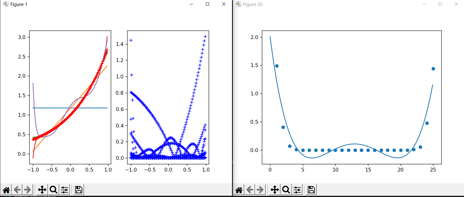
可能是由于不同软件的计算精度存在差异,上机实验中,在k分别取1,3,5,10时,并没有发现最大误差逐渐变大。但是,当我们进一步增大k至25以后,可以发现明显的计算异常,显然是由于计算机的舍入误差不断累积造成的异常结果。
## 第一个函数 1
2
3
4
5
6
7
8
9
10
11
12
13
14
15
16
17
18
19
20
21
22
23
24
25
26
27
28
29
30
31
32
33
34
35
36
37
38
39
40
41
42
43
44
45
46
47
48
49
50
51
52
53
54
55
56
57
58
59
60
61
62
63
64
65
66
67
68
69
70
71
72
73
74
75
76# 最佳平方逼近多项式 $f1
import numpy as np
import sympy as sp
from matplotlib import pyplot as plt
def gauss(a,b,k):
A = np.zeros((k+1,k+1))
x = sp.symbols("x")
for i in range(k+1):
for j in range(k+1):
A[i,j]=sp.integrate(x**(i+j),(x,a,b))
return A
def d(a,b,k):
B = np.zeros((k+1,1))
x = sp.symbols("x")
for i in range(k+1):
B[i,0]=sp.integrate(sp.E**x*x**i,(x,a,b))
#print(sp.E**x*x**i)
return B
def draw_fit(C,a,b,n,k):
#plt.figure(k+1)
# 拟合曲线
X = np.arange(a,b,1/n)
Y = []
plt.subplot(1,2,1)
for x in X:
sum = 0
for i in range(k+1):
sum = sum + C[i]*pow(x,i)
#print(type(sum.tolist()))
Y.append(sum.tolist()[0][0])
plt.plot(X,Y)
# 散点图
for x in np.arange(a,b,1/n):
y = np.exp(x)
plt.plot(x,y,"r+")
plt.subplot(1,2,2)
# 误差图
i=0
max = 0
for x in np.arange(a,b,1/n):
y = np.exp(x)
#print(y,Y[i],y-Y[i])
bias = abs(y-Y[i])
plt.plot(x,bias,"b+")
i += 1
if max < bias:
max = bias
return max
a = -1
b = 1 # 区间[-1,1]
n = 50
s = 25 # 图的个数
MAX = []
# 作图
for k in range(s):
G = gauss(a,b,k) # 法矩阵
D = d(a,b,k) # 法方程右边
G = np.matrix(G)
C = G.I.dot(D) # 法方程的解
MAX.append(draw_fit(C,a,b,n,k))
S = np.arange(1,s+1,1)
plt.figure(s+1)
plt.scatter(S,MAX)
# 最小二乘
z = np.polyfit(S,MAX,5)
p = np.poly1d(z)
xx = np.arange(0,s,0.1)
yy = p(xx)
plt.plot(xx,yy)
plt.show()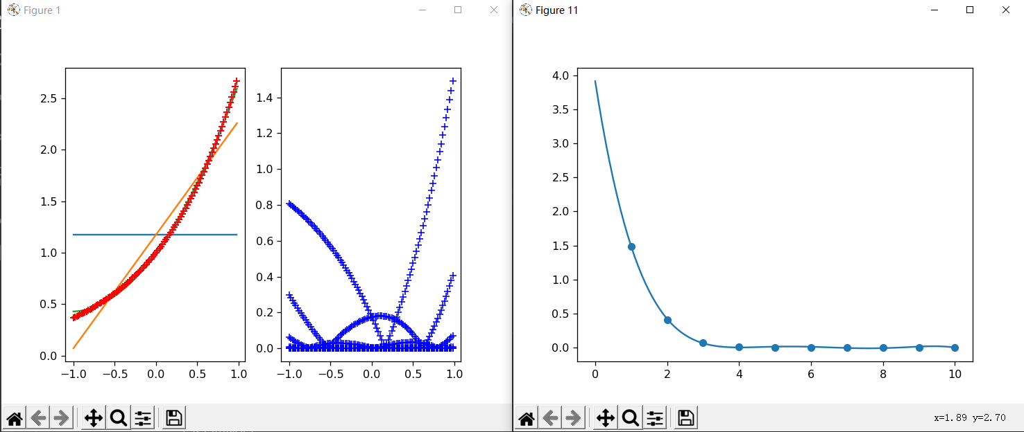 ### s=25 (k从0取到25)
 (注1:右图的曲线是最小二乘拟合的,散点为不同阶的最大误差)
(注2:继续增大代码的s,如s=30时,结果已经完全不可信,最大误差已经是几百几千了)
(注1:右图的曲线是最小二乘拟合的,散点为不同阶的最大误差)
(注2:继续增大代码的s,如s=30时,结果已经完全不可信,最大误差已经是几百几千了)
第二个函数
1 | # 最佳平方逼近多项式 # f2 |
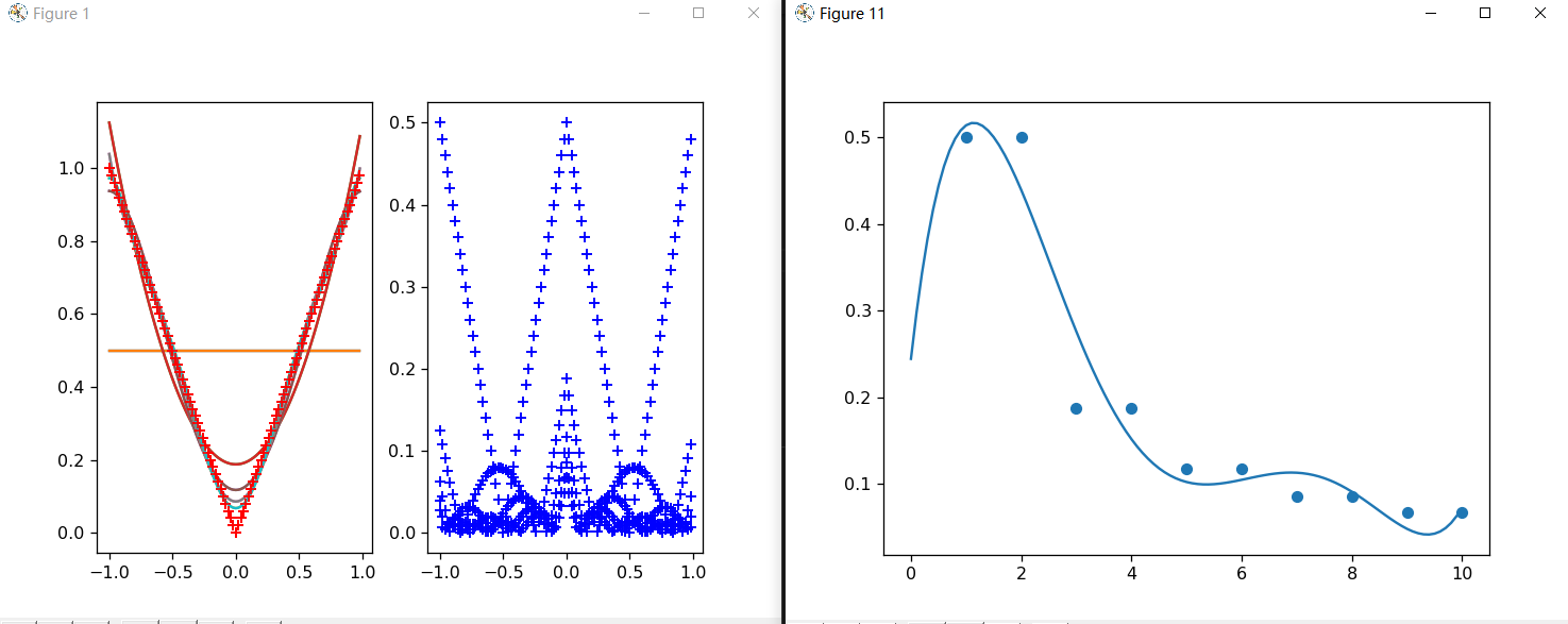
s=10 (k从0取到10)
 ### s=25 (k从0取到25)
 (注:s大于25后,也出现了最大误差上升) # 练习 二 (正交多项式的应用)
通过实验,我发现不管使用哪种方法计算,所得的结果都是一样的,代码中已经修改过不同计算方式所得曲线的颜色,报告中由于是黑白无法体现出来。观察误差图,可以发现三种方式得到的误差图是一模一样的。
(注:s大于25后,也出现了最大误差上升) # 练习 二 (正交多项式的应用)
通过实验,我发现不管使用哪种方法计算,所得的结果都是一样的,代码中已经修改过不同计算方式所得曲线的颜色,报告中由于是黑白无法体现出来。观察误差图,可以发现三种方式得到的误差图是一模一样的。
不过,虽然计算结果都是一样的,但是计算的效率却不相同,直观感受上,使用Chebyshev正交多项式的计算时长明显大于另外两个,而第一个的计算速度是最快的。分析可能存在两个影响因素:1.可能是由于计算机对多项式的处理速度比较快;2.从我的代码中可以发现,大量使用了计算库(numpy,sympy,scipy)的函数。事实上,如果通过递推公式,或者已知的两种正交多项式的正交性去计算,可以大量节省计算成本。(为了代码的复用性,我一开始并没打算这样做,但完成后发现了计算速度比较缓慢,故给出反思分析)
可以发现三者的代码是非常相似的。 ## 基函数 1
2
3
4
5
6
7
8
9
10
11
12
13
14
15
16
17
18
19
20
21
22
23
24
25
26
27
28
29
30
31
32
33
34
35
36
37
38
39
40
41
42
43
44
45
46
47
48
49
50
51
52
53
54
55
56
57
58
59
60
61
62
63
64
65
66
67
68
69
70
71
72# 正交多项式的应用
# 朴实无华基函数
import numpy as np
import sympy as sp
from matplotlib import pyplot as plt
def gauss(a,b,k):
A = np.zeros((k+1,k+1))
x = sp.symbols("x")
for i in range(k+1):
for j in range(k+1):
A[i,j]=sp.integrate(x**(i+j),(x,a,b))
return A
def d(a,b,k):
print(k)
B = np.zeros((k+1,1))
x = sp.symbols("x")
for i in range(k+1):
B[i,0]=sp.integrate(4/(4+25*(x+1)**2)*x**i,(x,a,b))
return B
def draw_fit(C,a,b,n,k):
plt.figure(k+1)
# 拟合曲线
X = np.arange(a,b,1/n)
Y = []
plt.subplot(1,2,1)
for x in X:
sum = 0
for i in range(k+1):
sum = sum + C[i]*pow(x,i)
#print(type(sum.tolist()))
Y.append(sum.tolist()[0][0])
plt.plot(X,Y)
# 散点图
for x in np.arange(a,b,1/n):
y = 4/(4+25*pow((x+1),2))
plt.plot(x,y,"r+")
plt.subplot(1,2,2)
# 误差图
i=0
max = 0
for x in np.arange(a,b,1/n):
y = 4/(4+25*pow((x+1),2))
#print(y,Y[i],y-Y[i])
bias = abs(y-Y[i])
plt.plot(x,bias,"b+")
i += 1
if max < bias:
max = bias
return max
a = -1
b = 1 # 区间[-1,1]
n = 50
s = 2 # 图的个数
MAX = []
# 作图
for k in [5,10]:
G = gauss(a,b,k) # 法矩阵
D = d(a,b,k) # 法方程右边
G = np.matrix(G)
C = G.I.dot(D) # 法方程的解
print(C)
MAX.append(draw_fit(C,a,b,n,k))
S = np.arange(1,s+1,1)
plt.figure(s+1)
plt.scatter(S,MAX)
plt.show()1
2
3
4
5
6
7
8
9
10
11
12
13
14
15
16
17
18
19
20
21
22
23
24
25
26
27
28
29
30
31
32
33
34
35
36
37
38
39
40
41
42
43
44
45
46
47
48
49
50
51
52
53
54
55
56
57
58
59
60
61
62
63
64
65
66
67
68
69
70
71
72
73
74
75
76
77
78
79
80
81
82
83
84
85
86
87
88
89
90
91
92
93
94
95# Legendre 正交多项式
import sympy as sp
import scipy as sc
import numpy as np
from math import factorial
from matplotlib import pyplot as plt
np.set_printoptions(suppress=True)
def gauss(a,b,k):
A = np.zeros((k+1,k+1))
x = sp.symbols("x")
f = 4/(4+25*(x+1)**2)
for i in range(k+1):
for j in range(k+1):
phi = (1/(2**i*factorial(i)))*sp.diff((x**2-1)**i,x,i)
phj = (1/(2**j*factorial(j)))*sp.diff((x**2-1)**j,x,j)
rho = 1
l = sp.integrate(rho*phi*phj,(x,a,b))
A[i,j]=l
#print(sp.expand(phi)) #测试正交多项式
#print(sp.Rational(sp.expand(phi).coeff(x**4))) #测试系数
#print(A) #测试法矩阵
return A
def d(a,b,k):
print(k)
B = np.zeros((k+1,1))
x = sp.symbols("x")
f = 4/(4+25*(x+1)**2)
rho = 1
for i in range(k+1):
phi = (1/(2**i*factorial(i)))*sp.diff((x**2-1)**i,x,i)
g = f*phi*rho
g = sp.lambdify([x], g) #匿名函数化
l=sc.integrate.quad(g,a,b)[0] #为避免报错采用数值积分
B[i,0]=l
return B
def draw_fit(C,a,b,n,k):
plt.figure(k+1)
# 拟合曲线
X = np.arange(a,b,1/n)
Y = []
plt.subplot(1,2,1)
x = sp.symbols("x")
for t in X:
sum = 0
for i in range(k+1):
phi = (1/(2**i*factorial(i)))*sp.diff((x**2-1)**i,x,i)
sum = sum + C[i]*phi.evalf(subs ={'x':t})
#print(type(sum.tolist()))
Y.append(sum.tolist()[0][0])
plt.plot(X,Y)
# 散点图
for x in np.arange(a,b,1/n):
y = 4/(4+25*pow((x+1),2))
plt.plot(x,y,"r+")
plt.subplot(1,2,2)
# 误差图
i=0
max = 0
for x in np.arange(a,b,1/n):
y = 4/(4+25*pow((x+1),2))
#print(y,Y[i],y-Y[i])
bias = abs(y-Y[i])
plt.plot(x,bias,"b+")
i += 1
if max < bias:
max = bias
return max
a = -1
b = 1 # 区间[-1,1]
n = 50
s = 2 # 图的个数
MAX = []
# 作图
for k in [5,10]:
G = gauss(a,b,k) # 法矩阵
D = d(a,b,k) # 法方程右边
print(D)
G = np.matrix(G)
C = G.I.dot(D) # 法方程的解
print(C)
MAX.append(draw_fit(C,a,b,n,k))
S = np.arange(1,s+1,1)
plt.figure(s+1)
plt.scatter(S,MAX)
plt.show()1
2
3
4
5
6
7
8
9
10
11
12
13
14
15
16
17
18
19
20
21
22
23
24
25
26
27
28
29
30
31
32
33
34
35
36
37
38
39
40
41
42
43
44
45
46
47
48
49
50
51
52
53
54
55
56
57
58
59
60
61
62
63
64
65
66
67
68
69
70
71
72
73
74
75
76
77
78
79
80
81
82
83
84
85
86
87
88
89
90
91
92
93
94
95# Chebyshev 正交多项式
import sympy as sp
import scipy as sc
import numpy as np
from math import factorial
from matplotlib import pyplot as plt
np.set_printoptions(suppress=True)
def gauss(a,b,k):
A = np.zeros((k+1,k+1))
x = sp.symbols("x")
f = 4/(4+25*(x+1)**2)
for i in range(k+1):
for j in range(k+1):
phi = sp.cos(i*sp.acos(x))
phj = sp.cos(j*sp.acos(x))
rho = 1
l = sp.integrate(rho*phi*phj,(x,a,b))
A[i,j]=l
#print(sp.expand(phi)) #测试正交多项式
#print(sp.Rational(sp.expand(phi).coeff(x**4))) #测试系数
#print(A) #测试法矩阵
return A
def d(a,b,k):
print(k)
B = np.zeros((k+1,1))
x = sp.symbols("x")
f = 4/(4+25*(x+1)**2)
rho = 1
for i in range(k+1):
phi = sp.cos(i*sp.acos(x))
g = f*phi*rho
g = sp.lambdify([x], g) # 匿名函数化
l=sc.integrate.quad(g,a,b)[0] # 为避免报错采用数值积分
B[i,0]=l
return B
def draw_fit(C,a,b,n,k):
plt.figure(k+1)
# 拟合曲线
X = np.arange(a,b,1/n)
Y = []
plt.subplot(1,2,1)
x = sp.symbols("x")
for t in X:
sum = 0
for i in range(k+1):
phi = sp.cos(i*sp.acos(x))
sum = sum + C[i]*phi.evalf(subs ={'x':t})
#print(type(sum.tolist()))
Y.append(sum.tolist()[0][0])
plt.plot(X,Y,"g")
# 散点图
for x in np.arange(a,b,1/n):
y = 4/(4+25*pow((x+1),2))
plt.plot(x,y,"r+")
plt.subplot(1,2,2)
# 误差图
i=0
max = 0
for x in np.arange(a,b,1/n):
y = 4/(4+25*pow((x+1),2))
#print(y,Y[i],y-Y[i])
bias = abs(y-Y[i])
plt.plot(x,bias,"b+")
i += 1
if max < bias:
max = bias
return max
a = -1
b = 1 # 区间[-1,1]
n = 50
s = 2 # 图的个数
MAX = []
# 作图
for k in [5,10]:
G = gauss(a,b,k) # 法矩阵
D = d(a,b,k) # 法方程右边
print(D)
G = np.matrix(G)
C = G.I.dot(D) # 法方程的解
print(C)
MAX.append(draw_fit(C,a,b,n,k))
S = np.arange(1,s+1,1)
plt.figure(s+1)
plt.scatter(S,MAX)
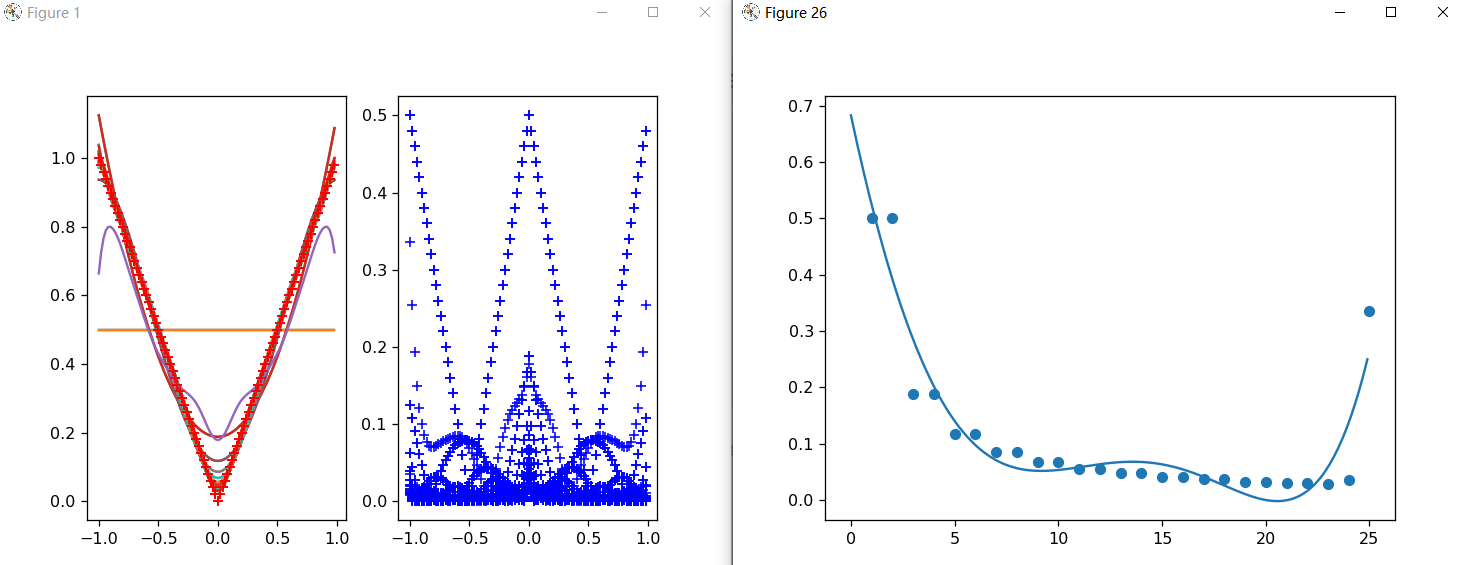
plt.show()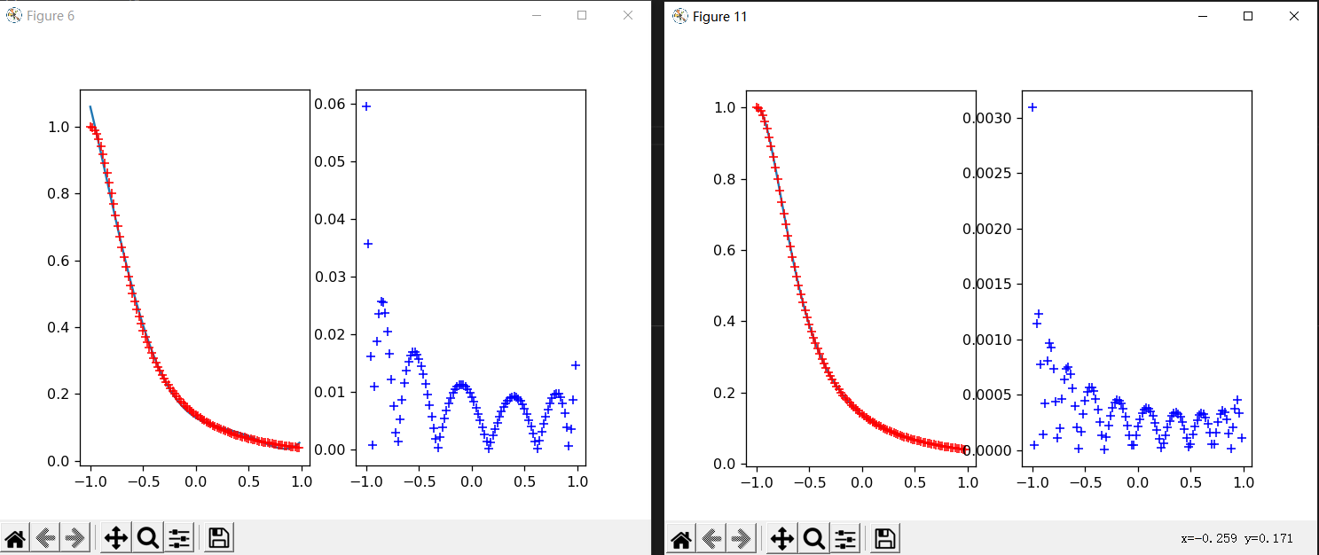 左图为k=5,右图为k=10.
k=5的最佳逼近多项式系数 [[ 0.12885774] [-0.19746297] [ 0.44698082]
[-0.61910836] [-0.01585597] [ 0.3170046 ]] k=10的最佳逼近多项式系数 [[
0.13771554] [-0.24145138] [ 0.30710191] [-0.22830788] [ 0.07656059]
[-0.52033777] [ 0.83695426] [ 0.47672007] [-1.18338108] [ 0.03469561] [
0.34327799]]
另外,可以发现选择正交多项式求解时,k的增加不会改变法方程解前面的项,只需要在后面增加一项即可,如果在代码中实现,也将大幅减少计算量。最关键的是使用正交多项式求解可以避免,病态线性方程组的求解。
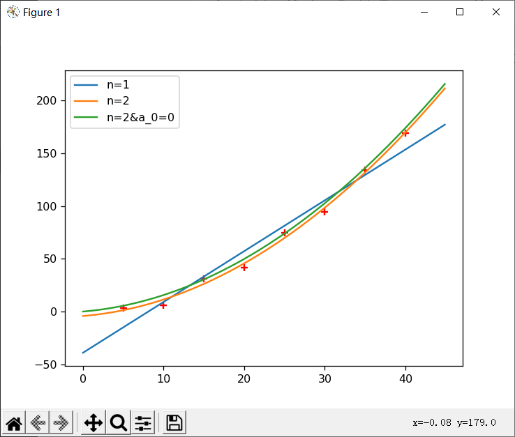
# 练习 三(多项式最小二乘法) ## 分析
效果上看第三种拟合最符合实际,因为汽车的初速度为0时,刹车距离自然为0. ##
代码
左图为k=5,右图为k=10.
k=5的最佳逼近多项式系数 [[ 0.12885774] [-0.19746297] [ 0.44698082]
[-0.61910836] [-0.01585597] [ 0.3170046 ]] k=10的最佳逼近多项式系数 [[
0.13771554] [-0.24145138] [ 0.30710191] [-0.22830788] [ 0.07656059]
[-0.52033777] [ 0.83695426] [ 0.47672007] [-1.18338108] [ 0.03469561] [
0.34327799]]
另外,可以发现选择正交多项式求解时,k的增加不会改变法方程解前面的项,只需要在后面增加一项即可,如果在代码中实现,也将大幅减少计算量。最关键的是使用正交多项式求解可以避免,病态线性方程组的求解。
# 练习 三(多项式最小二乘法) ## 分析
效果上看第三种拟合最符合实际,因为汽车的初速度为0时,刹车距离自然为0. ##
代码 1
2
3
4
5
6
7
8
9
10
11
12
13
14
15
16
17
18
19
20
21
22
23
24
25
26
27
28
29
30
31
32
33
34
35
36
37
38
39
40
41
42
43
44
45
46
47
48
49# 多项式的最小二乘法
import numpy as np
from matplotlib import pyplot as plt
# 数据及散点图
X = [5,10,15,20,25,30,35,40]
Y = [3.42,5.96,31.14,41.76,74.54,94.32,133.78,169.16]
plt.scatter(X,Y,marker='+',c='r')
def match(n,X,Y):
l = len(X)
A = np.zeros((n+1,n+1))
B = np.zeros(n+1)
for i in range(n+1): # 法矩阵
for j in range(n+1):
sum = 0
for k in range(l):
sum = sum + pow(X[k],i+j)
A[i,j]=sum
for i in range(n+1): # 法方程右边
for j in range(n+1):
sum = 0
for k in range(l):
sum = sum + pow(X[k],i)*Y[k]
B[i]=sum
A = np.matrix(A)
C = A.I.dot(B) # 系数向量
C = np.array(C)
return C
# 一次拟合
C = match(1,X,Y)
xx = np.arange(0,45,0.1)
yy = C[0,1] * xx + C[0,0]
plt.plot(xx,yy,label='n=1')
# 二次拟合
C = match(2,X,Y)
yy = C[0,2] * np.power(xx,2) + C[0,1] * xx + C[0,0]
plt.plot(xx,yy,label='n=2')
# 无常数项拟合
C = match(2,X,Y)
yy = C[0,2] * np.power(xx,2) + C[0,1] * xx
plt.plot(xx,yy,label='n=2&a_0=0')
plt.legend()
plt.show()
运行结果
练习 四 (指数函数最小二乘法)
代码
1 | # 指数函数的最小二乘法 |
运行结果
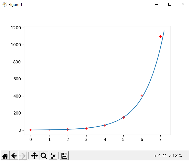 ## 结果分析
从图像上不容易看出,但在k=7时的绝对误差已经是几十的数量级了,但是相对误差还是比较小的。
## 结果分析
从图像上不容易看出,但在k=7时的绝对误差已经是几十的数量级了,但是相对误差还是比较小的。